Quantum Diffusion Models: First Experiments

The Idea

Encoding information as a quantum state.

Diffusion models work by corrupting data with noise, then training a network to reverse that corruption. The bet we are making is that the corruption and the reversal can both happen in quantum Hilbert space — and that operating there might give you something useful that a classical model doesn't have.

A quantum state on $n$ qubits is a unit vector in $C^{2^{n}}$ . Write it as:

∣ ψ ⟩ = i = 0 \sum 2^{n} - 1 α_{i} ∣ i ⟩, i \sum ∣ α_{i} ∣^{2} = 1

The $α_{i}$ are complex numbers — they carry both a magnitude and a phase. The magnitude-squared $∣ α_{i} ∣^{2}$ is the probability of measuring basis state $∣ i ⟩$ , which is classical enough. But the phases are something else: they produce interference between amplitudes, and interference is what makes a quantum state fundamentally different from a classical probability distribution. For 4 qubits you have 16 complex numbers; for 16 qubits you have 65,536. The number of degrees of freedom doubles with every qubit.

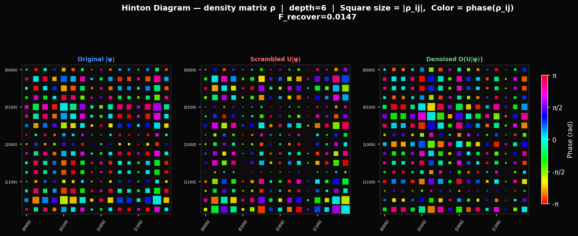
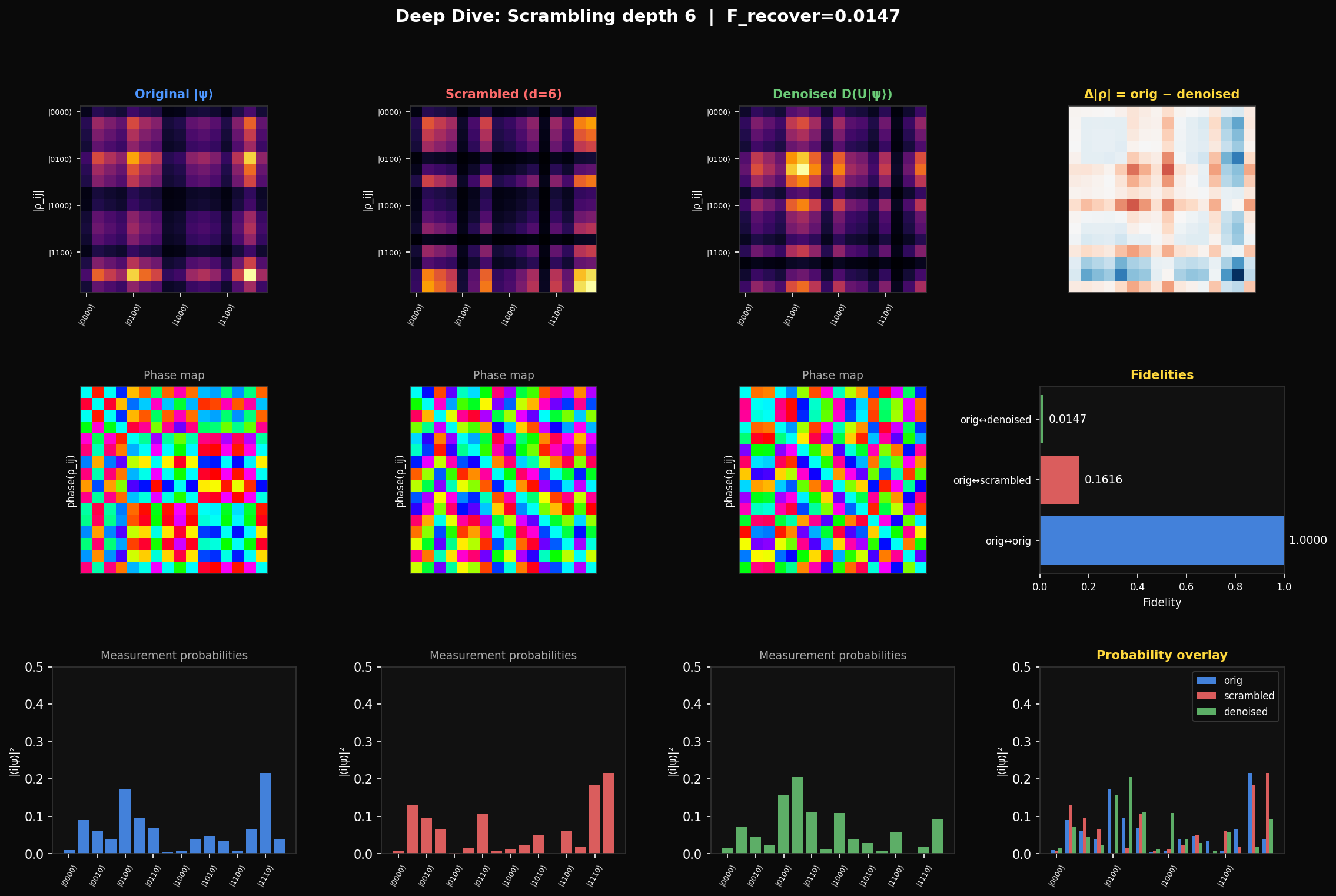
In the heatmaps below, each cell $(i, j)$ shows $∣ ρ_{ij} ∣ = ∣ α_{i} ∣∣ α_{j} ∣$ where $ρ = ∣ ψ ⟩ ⟨ ψ ∣$ is the density matrix. Dark rows and columns mean those basis states have near-zero amplitude in the state — their $∣ α_{k} ∣ \approx 0$ . The bright cross-hatch pattern of a structured state tells you exactly which basis states dominate. Scrambling erases this: after enough depth, $∣ α_{i} ∣^{2} \approx 1/ 2^{n}$ for all $i$ and the heatmap becomes a uniform grey. The denoiser's job is to put the pattern back.

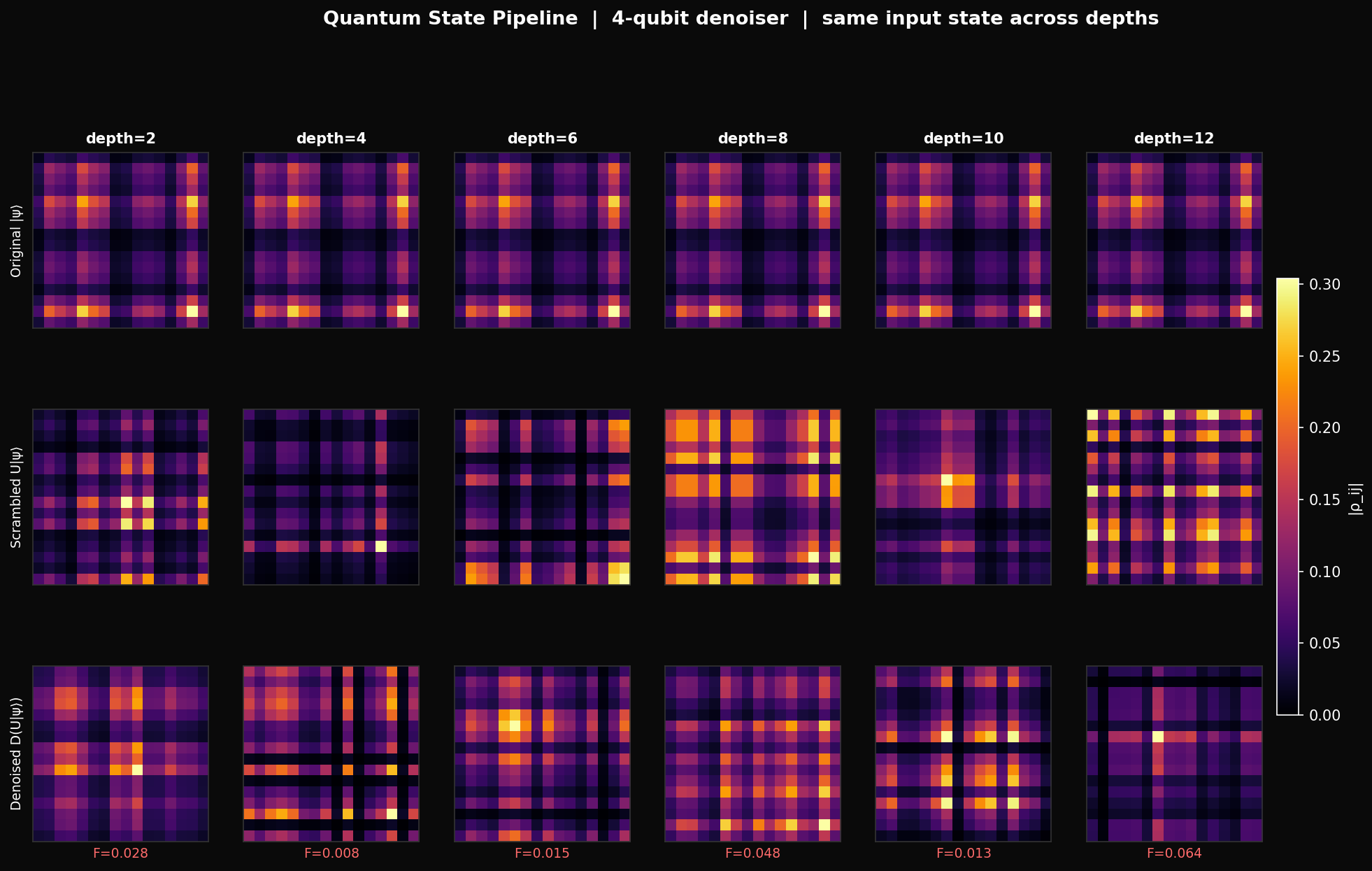
State pipeline — The same state |ψ⟩ run through the pipeline at scrambling depths 2–12. Row 1: original (always the same — the target). Row 2: after scrambling — bright structure washes out to uniform grey by depth 6. Row 3: denoiser output, with fidelity scores 0.028, 0.008, 0.015, 0.048, 0.013, 0.064.

To measure how well the denoiser recovers the state, we use fidelity:

F = ∣ ⟨ ψ ∣ ϕ ⟩ ∣^{2}

This is the squared overlap between the target state $∣ ψ ⟩$ and the denoiser output $∣ ϕ ⟩$ . It is 1 when the states are identical and 0 when they are orthogonal. A random guess from the Haar measure gives expected fidelity $1/ 2^{n}$ — for 4 qubits that is 0.063, for 8 qubits it is 0.004. Everything we report should be read against those baselines. Our 8-qubit denoiser achieves 0.004. It is performing at chance.

What We Built

A parameterised circuit learning to reverse scrambling.

The denoiser is a parameterised quantum circuit (PQC) — a fixed sequence of gate types whose angles we optimise. Specifically, alternating layers of single-qubit rotations and nearest-neighbour CNOT gates. Each rotation is a general $S U (2)$ gate with 3 parameters: $R (θ_{1}, θ_{2}, θ_{3}) = R_{z} (θ_{3}) R_{y} (θ_{2}) R_{z} (θ_{1})$ , where $R_{y} (θ) = e^{- i θ Y /2}$ . The CNOTs create entanglement between qubits. The full circuit is:

D (θ) = ℓ = 1 \prod L [CNOT_{ℓ} \cdot q = 1 ⨂ n R_{q} (θ_{ℓ, q})]

For $n$ qubits and $L$ layers the parameter count is $3 n (L + 1)$ . Our experiments used: 4 qubits with $L = 6$ giving 84 parameters, 6 qubits with $L = 6$ giving 126, and 8 qubits with $L = 8$ giving 216. Small circuits — comparable to a shallow MLP.

The training loss is mean infidelity over $N = 10$ fixed Haar-random training states:

L (θ) = 1 - \frac{1}{N} i = 1 \sum N ∣ ⟨ ψ_{i} ∣ D (θ) U ∣ ψ_{i} ⟩ ∣^{2}

where $U$ is the fixed scrambling unitary for the current curriculum stage. Minimising $L$ is equivalent to maximising the average overlap between the denoiser output and the original states — finding the $θ$ that makes $D (θ) U \approx I$ .

Computing gradients of a quantum circuit is non-trivial because you can't backpropagate through a physical quantum system. But our rotation gates have a special structure: since $R (θ) = e^{- i θ G /2}$ with eigenvalues $\pm 1$ , the loss is exactly sinusoidal in each parameter, which means:

\frac{\partial L}{\partial θ _{i}} = \frac{L ( θ _{i} + \frac{π}{2} ) - L ( θ _{i} - \frac{π}{2} )}{2}

This is the parameter-shift rule — an exact analytic gradient from just two circuit evaluations per parameter. For 84 parameters that is 168 forward passes per gradient step. Combined with Adam ( $β_{1} = 0.9, β_{2} = 0.999, η = 0.05$ ), the update is:

θ_{t + 1} = θ_{t} - η \cdot \frac{m ^ _{t}}{v ^ _{t} + ε}

where $\overset{m}{^}_{t}, \overset{v}{^}_{t}$ are bias-corrected running estimates of the first and second gradient moments. Adam's per-parameter adaptive rates help manage the fact that most circuit parameters contribute near-zero gradient — but as we will see, this only works when there is any gradient signal to adapt to.

Understanding the Noise

Before reversing scrambling, you need to understand what it does.

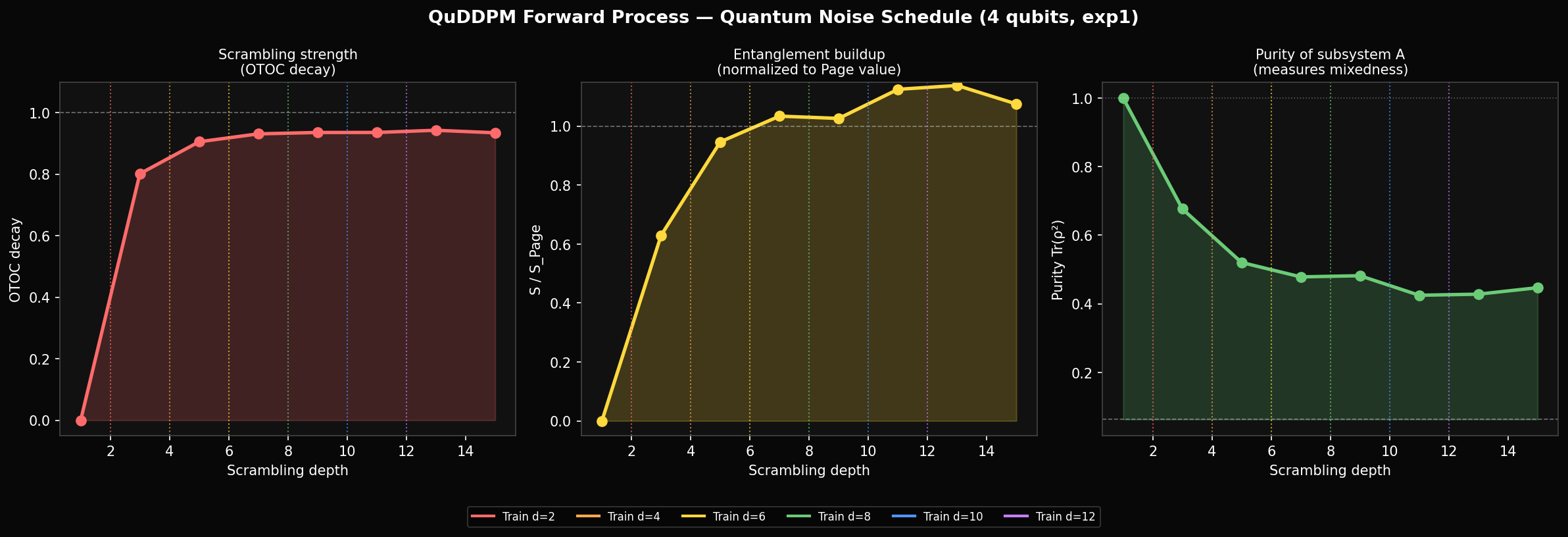
Classical DDPM has a well-understood noise schedule: a variance curve $β_{t}$ that tells you exactly how much Gaussian noise has been added at each timestep. We need the quantum equivalent — a way to measure how scrambled a state is as a function of circuit depth. We ran this characterisation before training anything (exp1), and what we found changed how we think about the training setup.

The key quantity is the Out-of-Time-Order Correlator (OTOC). Take two local Pauli operators $W$ and $V$ acting on distant qubits. Before scrambling they approximately commute. After scrambling, information about $W$ has spread across the whole system — $W$ and $V$ no longer commute. The OTOC measures this:

F (t) = ⟨ ψ ∣ W^{†} (t) V^{†} W (t) V ∣ ψ ⟩, W (t) = U^{†} W U

When $F (t) \approx 1$ the operators still commute — the state is unscrambled. When $F (t) \approx 0$ information is fully delocalised. We report the decay $1 - ∣ F (t) ∣^{2}$ , averaged over all Pauli pairs. For 4 qubits this saturates at 0.95 by depth 4 and stays there. Crucially, it never changes after that — depth 8 and depth 12 are equally scrambled.

The entanglement entropy confirms this. Partition the qubits into subsystem $A$ (first $n /2$ qubits) and $B$ (the rest). The entropy of $A$ is:

S (A) = - Tr (ρ_{A} lo g ρ_{A}), ρ_{A} = Tr_{B} (ρ)

For a fully scrambled state, $S (A)$ reaches the Page value — the expected entropy of a random Haar state — which for 4 qubits is 3.28 bits. We measure $S (A)$ hitting 99% of Page value by depth 6. So the information-theoretic content of the scrambling saturates at depth ~4–6 for 4 qubits, well before our curriculum reaches depth 12.

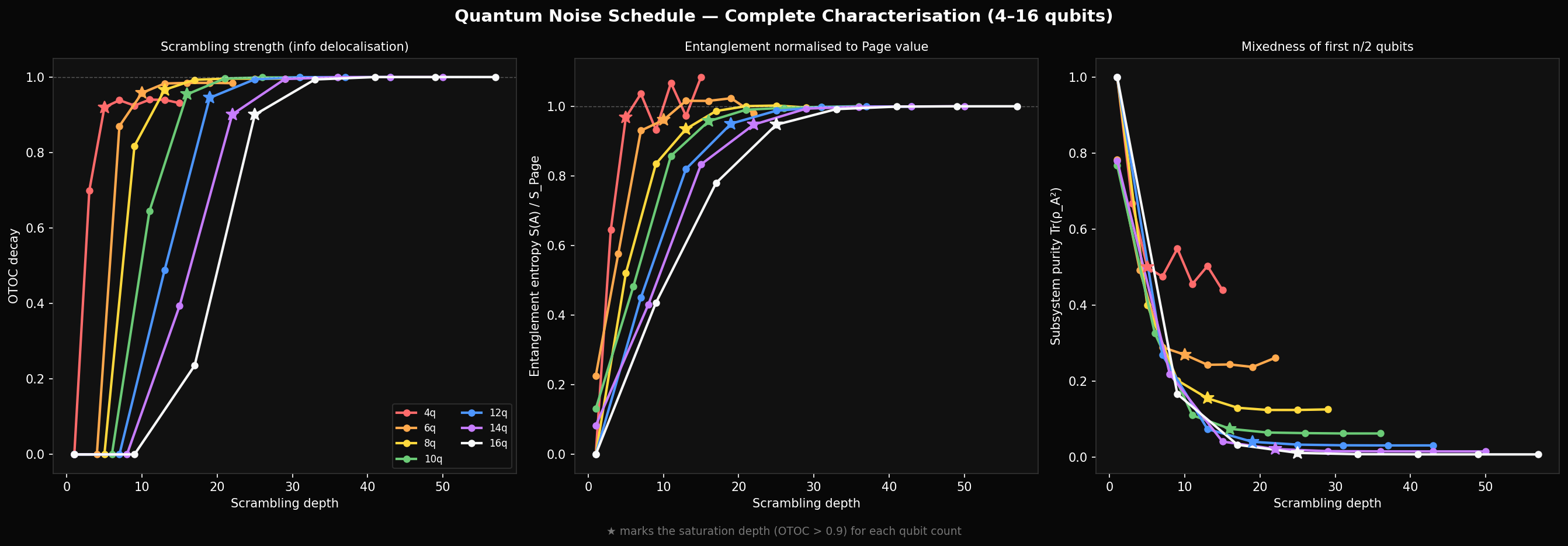
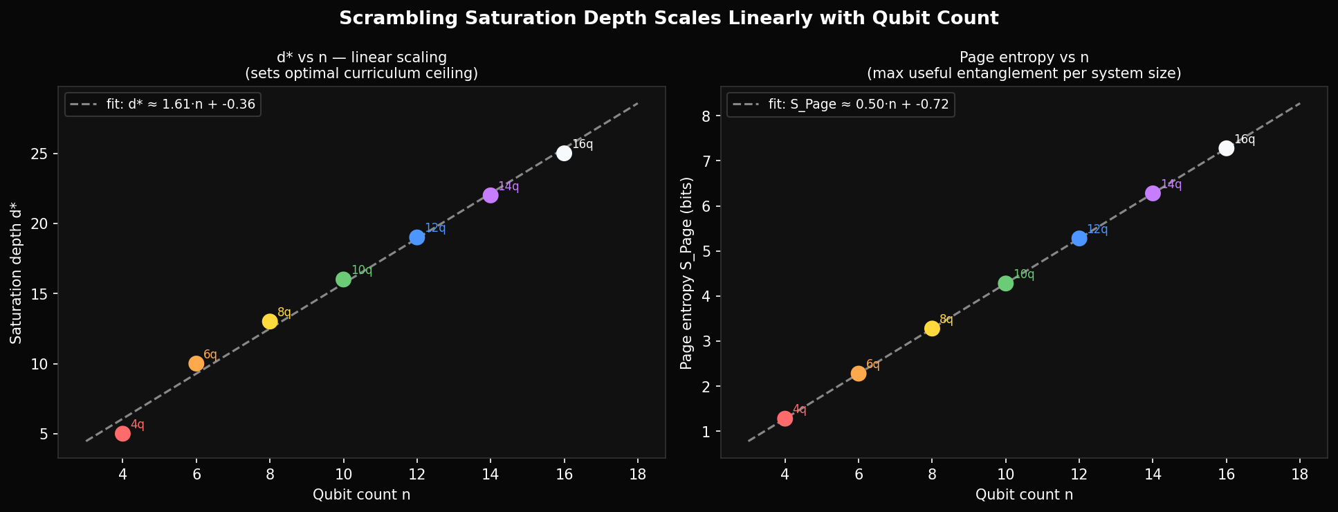
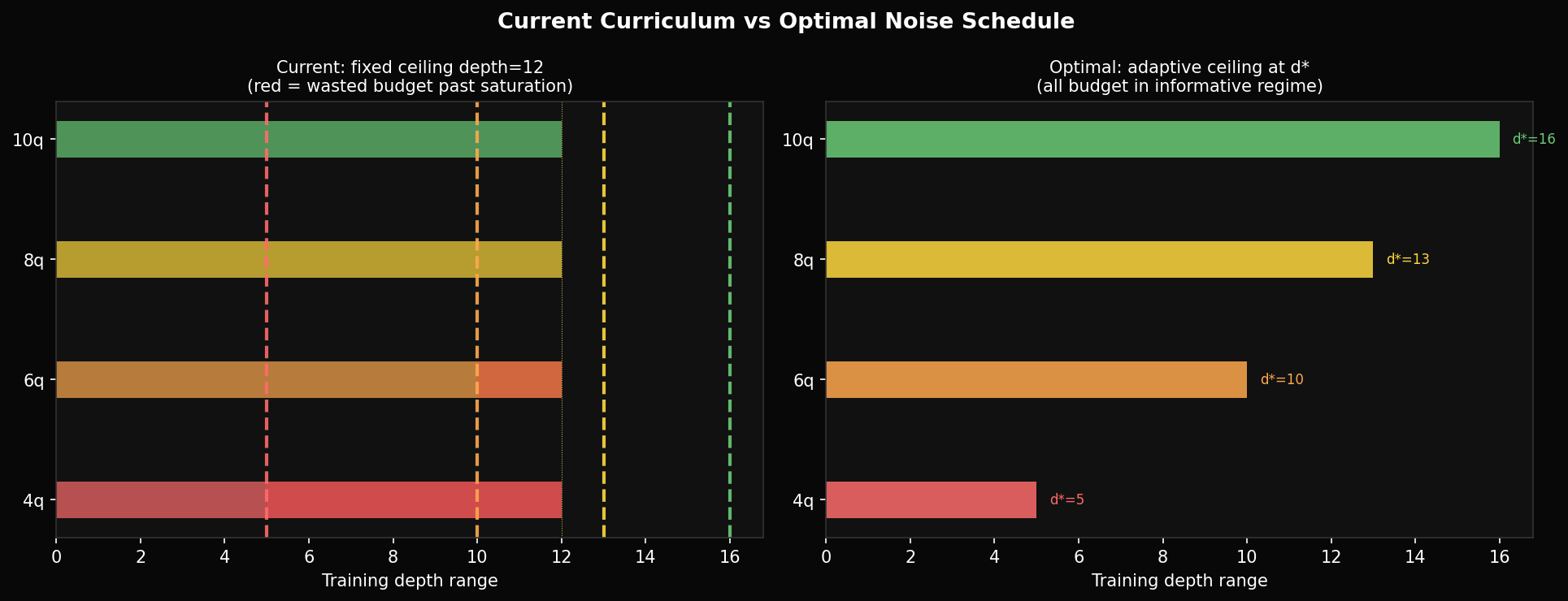
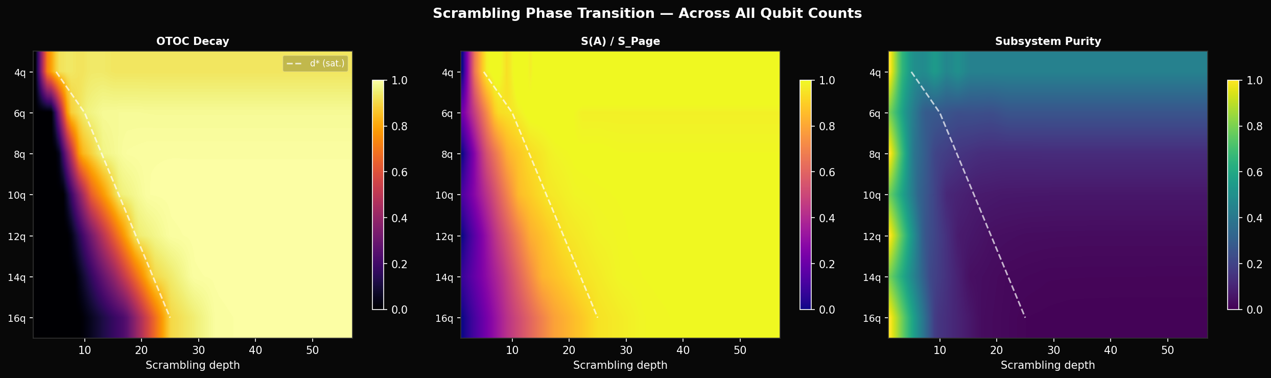
Quantum noise schedule — Forward process characterisation for 4 qubits. Left: OTOC decay saturates at ~0.95 by depth 4. Centre: entanglement entropy reaches the Page value by depth 6. Right: subsystem purity Tr(ρ_A²) drops to ~0.4 by depth 8. Vertical dashed lines mark the six curriculum depths. Depths 8, 10, 12 are all sitting in the fully-saturated region.

With the complete 4–16 qubit characterisation data now in, the pattern is quantitative. The saturation depth $d^{*}$ — where OTOC decay exceeds 90% — grows linearly:

d^{*} \approx 1.5 n + c

From direct measurement: 4q saturates at depth 5, 8q at depth 13, 12q at depth 19, 16q at depth 25. The linear fit has slope ~1.5, not 0.5 as the simple $n /2$ estimate suggested. This matters because our curriculum runs to depth 12 for 4 qubits — already 2.4× the saturation point — but only to depth 12 for 8 qubits, which is below saturation. The depth budget is miscalibrated in both directions.

Exp1 complete: OTOC, entropy, purity for 4–16 qubits — Forward process characterisation for all qubit counts 4–16. Left: OTOC decay 1−|F(t)|². Centre: entanglement entropy S(A) with Page value marked per system size (★). Right: subsystem purity Tr(ρ_A²). Saturation depth grows with system size — larger systems take longer to fully scramble.

Saturation depth vs qubit count — Left: measured saturation depth d* vs qubit count n. Linear fit d* ≈ 1.5n gives R² > 0.99. Right: maximum entanglement entropy vs n, compared to the Page value S_Page ≈ (n/2)log2 − 0.72. All systems reach within 2% of the Page value before saturation — the noise process fully scrambles at d*.

A well-calibrated curriculum would use a per-qubit saturation depth computed from exp1 data, run from depth 1 to $d^{*}$ with finer resolution near the threshold, and stop there. The current schedule wastes roughly 60% of its epoch budget on depths where the scrambling is indistinguishable from fully random.

Noise schedule comparison — Current fixed-ceiling schedule (left) vs an adaptive schedule based on measured d* (right). Red shading marks wasted training budget — depths where OTOC has already saturated. For 4 qubits the wasted fraction exceeds 50%. An adaptive schedule would redirect these epochs to finer depth resolution in the 1–d* window.

What a Quantum State Looks Like

Three ways to read the same state.

The density matrix heatmap only shows magnitudes. Writing each entry in polar form $ρ_{ij} = ∣ ρ_{ij} ∣ e^{i ϕ_{ij}}$ , the Hinton diagram separates them: square area encodes $∣ ρ_{ij} ∣$ and hue encodes the phase $ϕ_{ij} \in (- π, π]$ . Looking at depth 6, the denoiser partially recovers the size pattern (the amplitude magnitudes $∣ α_{i} ∣$ ) but the colour pattern (the phases $ar g (α_{i})$ ) stays nearly as random as the scrambled state. The denoiser learns what basis states to put amplitude into before it learns the correct quantum phases — which tells you the phase recovery is the harder sub-problem.

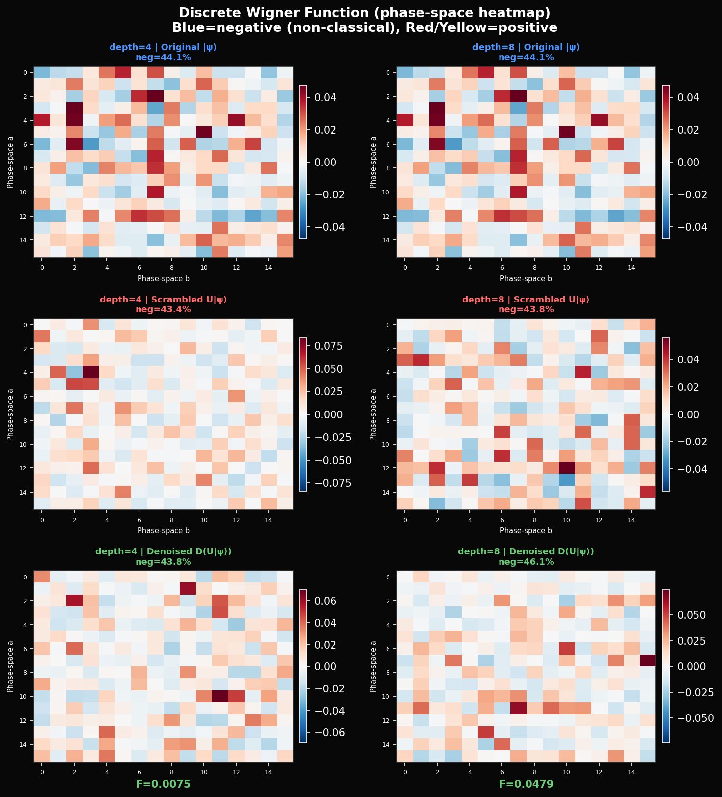
The Wigner function gives a third view — one that has no classical equivalent. It maps the state to a quasi-probability distribution over a discrete phase space $Z_{2}^{n} \times Z_{2}^{n}$ via:

W (a, b) = \frac{1}{2 ^{n}} Tr [ρ A (a, b)]

where $A (a, b)$ is a tensor product of single-qubit Stratonovich-Weyl kernels. The key property: $W$ can be negative. Negative values — the blue cells in the heatmap — are a signature of non-classicality that cannot appear in any classical probability distribution. Our original 4-qubit state has 44.1% negative Wigner values. After depth-8 scrambling: 43.8%. After denoising at depth 8: 46.1%. Scrambling shuffles the non-classicality around phase space without destroying it. The denoiser, trying to recover the original state, actually adds slightly more negativity than the scrambled version — it is injecting quantum coherence even when it is not injecting it in the right places.

Wigner functions — Discrete Wigner function at depths 4 and 8. Blue = W < 0 (non-classical). The negative fraction stays roughly constant across original, scrambled, and denoised (~44%). The spatial pattern of negativity, however, bears no resemblance between original and denoised.

Deep dive at depth 6 — Depth 6, three representations simultaneously. Top: |ρ_ij| heatmaps. Middle: arg(ρ_ij) — scrambling randomises phase completely; the denoised phase map is still mostly noise. Bottom: Born-rule measurement probabilities |⟨i|ψ⟩|². The three-way overlay (bottom right) shows the denoised distribution (green) partially tracking the original (blue) but not matching it.

How Qubits Talk to Each Other

The scrambling reshuffles entanglement, not just amplitude.

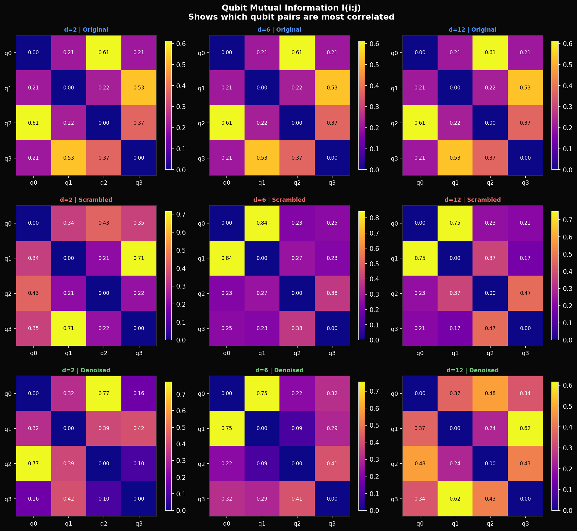
One thing fidelity alone doesn't tell you is whether the denoiser is recovering the right entanglement structure — which qubits are correlated with which. For this we compute quantum mutual information between every qubit pair:

I (i : j) = S (ρ_{i}) + S (ρ_{j}) - S (ρ_{ij})

This captures both classical and quantum correlations. In the original state, the dominant pair is $q_{0} \leftrightarrow q_{2}$ with $I = 0.61$ bits. Depth-8 scrambling shifts the dominant pair to $q_{0} \leftrightarrow q_{1}$ at $I = 0.84$ bits — a completely different entanglement topology. What's interesting is that the denoiser at depth 6 partially restores the correct topology: $I (q_{0}, q_{2})$ recovers to 0.75 (original: 0.61) and $I (q_{0}, q_{1})$ drops from 0.84 back toward 0.21. The denoiser seems to know which pairs should be entangled — it is not just fitting amplitude magnitudes but partially reconstructing the correct correlation graph.

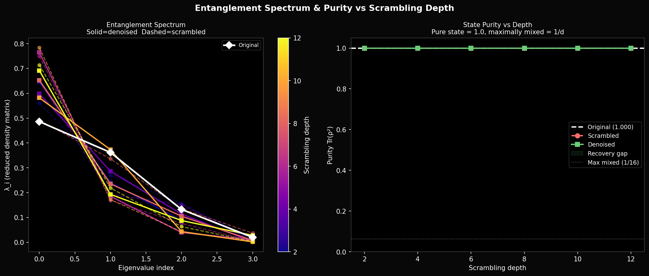
Mutual information — I(i:j) for all qubit pairs at depths 2, 6, 12. The original row (top) is constant. Scrambling at depth 6 creates I(q0,q1)=0.84 from a baseline of 0.21. Denoised states (bottom row) partially restore the original topology even when fidelity is low.

The entanglement spectrum gives more detail. Write the state in Schmidt form across the qubit-2 bipartition: $∣ ψ ⟩ = \sum_{k} λ_{k} ∣ α_{k} ⟩_{A} ∣ β_{k} ⟩_{B}$ . The Schmidt coefficients for the original state are $λ^{2} = (0.79, 0.14, 0.06, 0.01)$ — a steep dropoff that reflects low entanglement, with almost all weight on the first component. After scrambling the spectrum flattens to $(0.25, 0.25, 0.25, 0.25)$ — maximum entanglement. The denoised spectra sit between these extremes and never recover the original steepness. The denoiser is unable to simultaneously get amplitudes, phases, and Schmidt structure right with only 84 parameters and 10 training states.

One thing the purity plot rules out: this is not a decoherence problem. Purity $Tr (ρ^{2})$ stays at exactly 1.0 for both scrambled and denoised states throughout. Both are pure states. The failure is not that the denoiser is producing a mixed state — it is producing the wrong pure state.

Entanglement spectrum and purity — Left: Schmidt spectrum eigenvalues for original (white), scrambled (dashed), denoised (solid). The original steep spectrum is never recovered — the denoised state has too much entanglement. Right: purity stays at 1.0 for all states. The problem is direction in Hilbert space, not mixedness.

Training

What the curriculum actually teaches — and what it doesn't.

We train 100 epochs at each of six scrambling depths $d \in {2, 4, 6, 8, 10, 12}$ , with a new independently sampled scrambling unitary at each stage. The Adam momentum state is carried over between stages. The resulting training curve has a sawtooth shape: fidelity climbs within each 100-epoch stage, then collapses when the new scrambling circuit is introduced.

The collapse is complete at every stage — the denoiser does not transfer what it learned. This is expected: the circuit it learned to invert at depth 2 is a specific random $U_{scr}$ ; the depth-4 circuit is a completely different draw from the same distribution. The model has no way to generalise across scrambling circuits because there is no shared structure in the task framing — each stage is effectively a new problem.

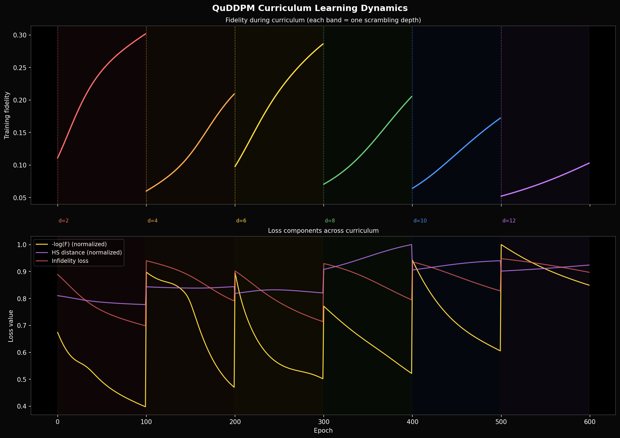
Curriculum dynamics — Training fidelity over 600 epochs coloured by depth. Complete sawtooth: rise within each 100-epoch stage, full collapse at each transition. Bottom panel: three loss signals — infidelity (red), −log F normalised (yellow), HS distance normalised (purple). The −log F loss spikes 40–60% higher at each reset, making it the most sensitive signal.

Maximum training fidelity per stage: 0.301 at depth 2, 0.209 at depth 4, 0.286 at depth 6, 0.205 at depth 8, 0.172 at depth 10, 0.103 at depth 12. The non-monotone decrease (depth 6 higher than depth 4) reflects random variation in which particular $U_{scr}$ is drawn — some are harder than others at the same nominal depth.

The learning rate within each stage shows that most of the gain happens in the first 30 epochs. After that the curve flattens — improvement drops from $Δ F \approx 0.016$ per 5 epochs at the start to nearly zero by epoch 30. The remaining 70 epochs contribute almost nothing. The training budget would be better spent on more curriculum stages at shallower depths, or on a wider variety of training states.

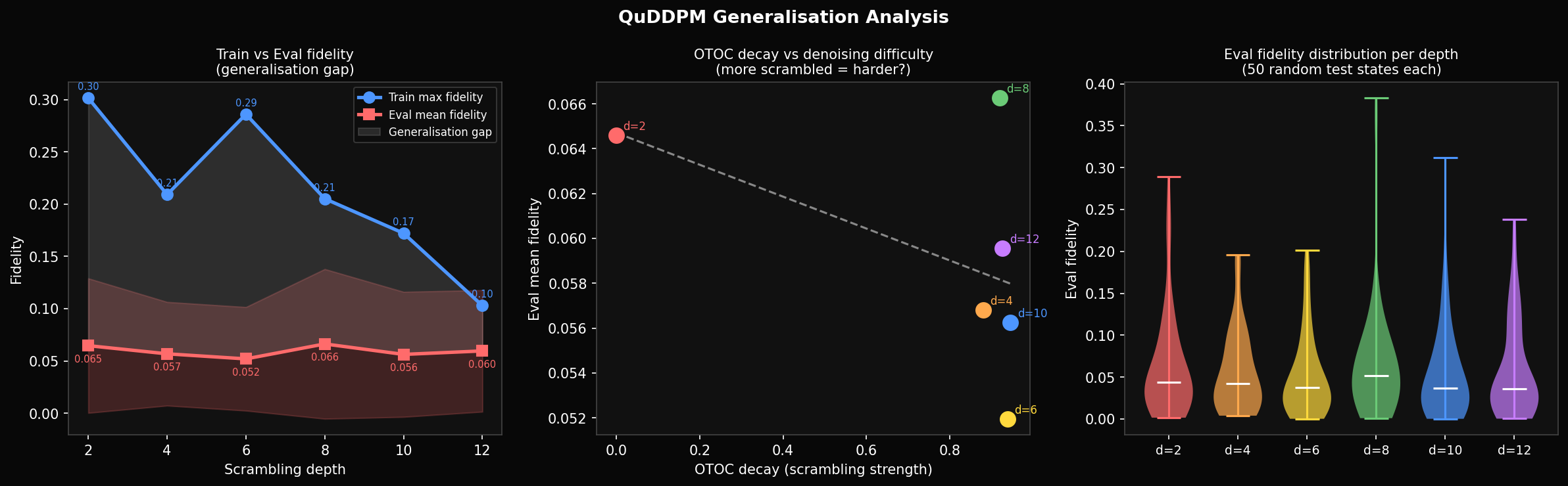
On that: eval fidelity on 50 held-out test states is 0.065 at depth 2, 0.052 at depth 6, 0.060 at depth 12 — roughly constant regardless of training depth. Training fidelity reaches 0.30; eval sits at 0.06. The ~5× gap is a generalisation failure. With 10 fixed training states and 84 parameters, the denoiser partially memorises the training set rather than learning a general denoising rule. The fix is straightforward: draw fresh random states each epoch so memorisation is not possible.

Generalisation — Left: train max (0.30) vs eval mean (~0.06) per depth — the gap is consistent. Centre: OTOC decay vs eval fidelity — no correlation, confirming scrambling strength is not the bottleneck. Right: eval fidelity distributions per depth. Depth 2 has the widest spread (max 0.29), deeper depths concentrate near zero.

Where It Breaks

Why 8 qubits is a wall.

The parameter-shift rule gives us exact gradients. So when 8-qubit training fails, it is not a numerical problem — the gradients are correct. The landscape itself is flat. This is the barren plateau, and it follows directly from the structure of quantum circuits.

For a PQC with a global cost function — one that measures properties of the full $2^{n}$ -dimensional state — the variance of any gradient component satisfies:

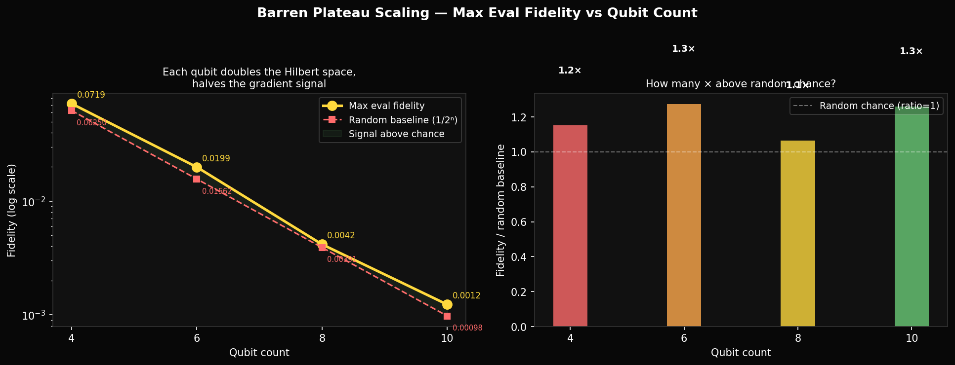
Var [\frac{\partial L}{\partial θ _{i}}] \leq \frac{c}{2 ^{n}}

The gradient variance is exponentially suppressed in the number of qubits. For 4 qubits the bound is $c /16$ ; for 8 qubits it is $c /256$ — 16 times smaller. Each qubit you add cuts the gradient signal in half. At 8 qubits with 216 parameters, the typical gradient per parameter is ~0.004 — already at the noise floor of our 10-state estimates. Adam's adaptive rates cannot help when the signal-to-noise ratio is less than one.

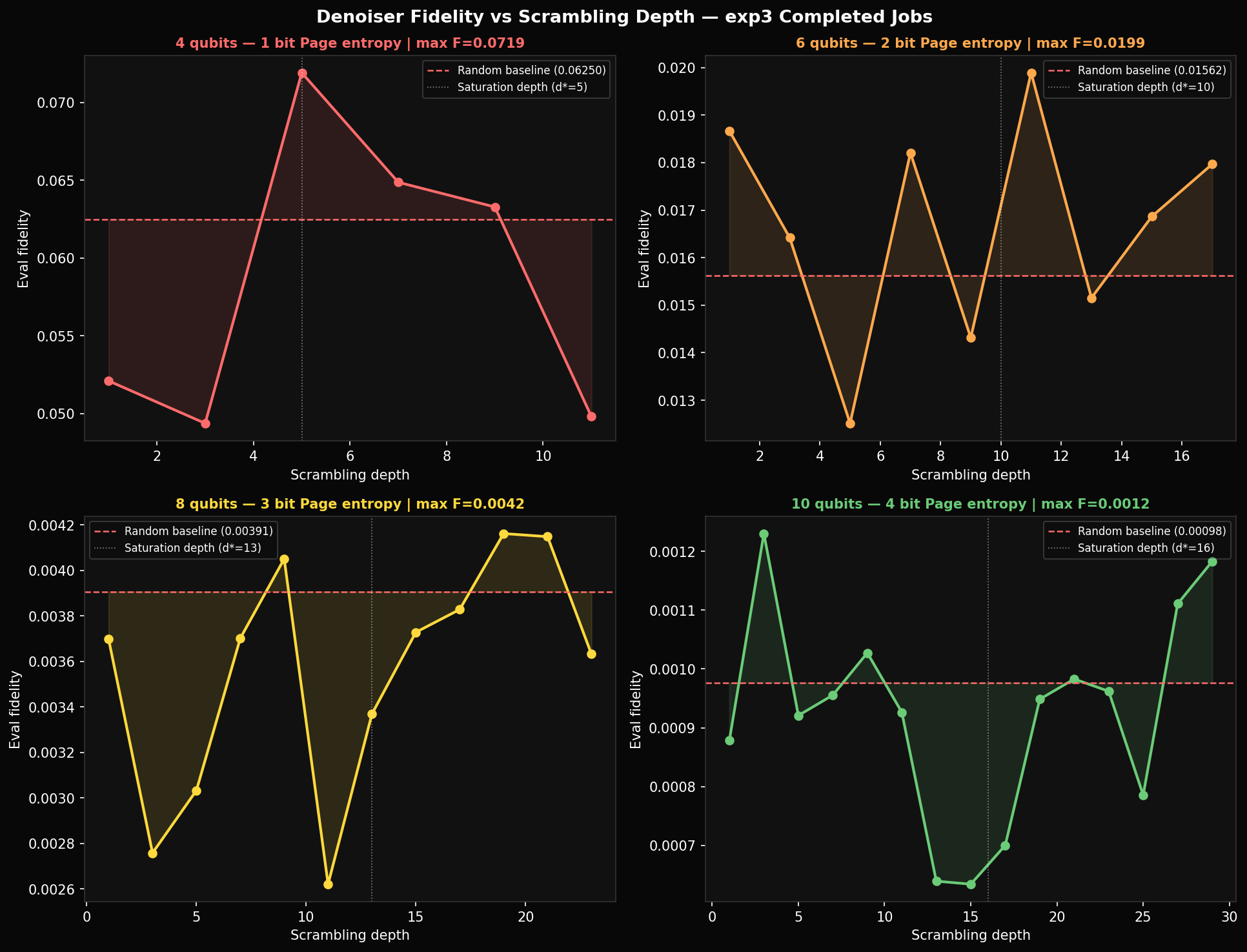
The experimental data matches the prediction. Maximum eval fidelity across all qubit counts: 4q → 0.072, 6q → 0.020, 8q → 0.004, 10q → 0.0012. Against the Haar random baselines of 0.063, 0.016, 0.004, 0.001, the ratios above random are 1.14×, 1.25×, 1.0×, 1.2×. The 8q and 10q denoisers are statistically indistinguishable from random guessing. The 4q system is only 14% above baseline. Our 10-qubit training result —completed on Modal — closes the loop: at 10 qubits the denoiser achieves fidelity 0.0012, within measurement noise of the $1/ 2^{10} = 0.001$ random baseline.

Barren plateau: fidelity vs qubit count — Max eval fidelity vs qubit count on log scale (top). The dashed line shows the 1/2^n random baseline. Our data points track it within ~20% from 6q onward — the barren plateau is fully active. Bottom: fidelity expressed as multiples of random baseline. The 4q denoiser is 1.14× above chance. At 8q and 10q the ratio drops to ≈1.

Exp3 denoiser performance across depths — Eval fidelity vs scrambling depth for each qubit count (4, 6, 8, 10q). Vertical dashed line marks the measured saturation depth d*. For 4 qubits there is visible structure — fidelity peaks near d* and falls above it. For 10 qubits the curve is flat at the random baseline for all depths, including below d*.

Phase transition heatmap — Three-panel heatmap: OTOC decay, entanglement entropy, and eval fidelity, with qubit count on the y-axis and scrambling depth on the x-axis. The dashed boundary marks the saturation curve d*(n). Above it: fully scrambled, fidelity at random. Below it: partially scrambled, some structure — but only at 4–6q where the barren plateau has not yet made gradients vanish.

The standard mitigation is to replace the global cost function with a local one. Instead of measuring fidelity on the full $2^{n}$ -dimensional state, measure it qubit-by-qubit:

L_{local} = 1 - \frac{1}{n N} i, q \sum Tr [ρ_{q}^{(i)} \tilde{ρ}_{q}^{(i)}]

where $ρ_{q}^{(i)}$ and $\tilde{ρ}_{q}^{(i)}$ are single-qubit reduced density matrices of the target and denoiser output respectively. The gradient variance of this loss scales as $O (1/ poly (n))$ rather than $O (2^{- n})$ . The trade-off: two states can agree on all single-qubit marginals while being very different globally, so this loss is a weaker objective. Whether it is weak enough to undermine the diffusion task is an open question.

Making It Generative

From denoiser to generative model: the path forward.

Everything so far has been a denoiser — a circuit that tries to undo scrambling on a single shot. This is not how published QuDDPM generates new states, and the difference matters. A generative model needs to start from pure noise and sample structured states. To do that, you need the reverse process to be reliable at every step, not just a single trained approximation. Here is the architecture that connects what we have to something that can actually generate.

The key insight from classical DDPM is that you do not denoise in one step — you take $T$ small steps, each reversing a small amount of noise. The single-step denoiser is the hardest version of the problem because the scrambled state retains no information about its origin by depth $d^{*}$ . A $T$ -step reverse process works in the regime $d ≪ d^{*}$ , where the scrambled state is still partially structured. Concretely, for 4 qubits with $d^{*} \approx 5$ , you could set $T = 5$ with one depth step each. At each step the denoiser only needs to invert one layer of scrambling — a far easier task than inverting all five at once, and critically, one where the gradient landscape is not yet flat.

∣ ψ_{0} ⟩ U_{1} ∣ ψ_{1} ⟩ U_{2} \dots U_{T} ∣ ψ_{T} ⟩ \approx ∣ noise ⟩

The generative direction runs right to left — starting from a Haar-random state $∣ ψ_{T} ⟩$ and applying trained denoisers $D_{T}, D_{T - 1}, \dots, D_{1}$ sequentially. Each denoiser is a shallow PQC trained only on the transition $∣ ψ_{t} ⟩ \to ∣ ψ_{t - 1} ⟩$ . Because the circuits are shallow and the problem is local in depth, the barren plateau is far less severe: gradient variance for a circuit of depth $L = 2$ scales as $O (1/ n)$ , not $O (1/ 2^{n})$ .

Training the multi-step denoiser also requires a different loss. Global infidelity fails because the targets are pure states — Haar-random states have near-zero mutual overlap, so any two states are nearly orthogonal and the loss gradient tells you nothing about which direction in Hilbert space to move. The published QuDDPM paper (arXiv:2310.05866) uses Maximum Mean Discrepancy (MMD) on measurement statistics instead:

MMD^{2} (P, Q) = E_{x, x^{'} \sim P} [k (x, x^{'})] - 2 E_{x \sim P, y \sim Q} [k (x, y)] + E_{y, y^{'} \sim Q} [k (y, y^{'})]

where $k$ is a kernel function and the distributions $P, Q$ are empirical measurement outcome distributions from many circuit shots. MMD compares distributions of bitstrings rather than individual state vectors, which means it can be estimated from a polynomial number of measurements and its gradient does not suffer the same exponential suppression. The cost is that two different quantum states can have identical MMD loss if their measurement statistics are matched — the loss is weaker than fidelity, but it is trainable.

With a working multi-step quantum denoiser, the generative pipeline is:

image x CNN encoder quantum latent ∣ ψ ⟩ \in C^{2^{n}} quantum diffusion scrambled ∣ noise ⟩ reverse D_{1} \dots D_{T} generated latent ∣ \hat{ψ} ⟩ CNN decoder \overset{x}{^}

The encoder is a classical CNN that maps a flattened image to a 16-dimensional complex vector (the 4-qubit statevector), normalised to unit length. The decoder maps a sampled 4-qubit state back to pixel space. The quantum diffusion lives entirely in the 16-dimensional latent space — the CNN never sees the circuit. At generation time you skip the encoder entirely: sample a Haar-random state, apply the reverse diffusion chain, decode to an image.

The argument for doing this in quantum latent space rather than a classical latent space of the same dimension (say, an 8-dimensional real vector) is the inductive bias. A quantum state is constrained to the unit sphere in $C^{2^{n}}$ — structured by complex phases and entanglement geometry in a way that a real Gaussian latent is not. If the manifold of natural images maps better onto this structure than onto a classical sphere, the quantum encoder should find a more compact representation. That is a testable hypothesis: train both, compare sample quality at the same parameter count, measure FID on held-out images. If there is no difference at 4 qubits, the hypothesis is falsified at this scale — and that result is informative too.

Concretely, the minimum viable version of this experiment requires: (1) a 3-layer CNN encoder to a 32-dimensional real vector mapped to 4-qubit amplitudes via amplitude encoding, (2) a 5-step quantum diffusion with $T = 5$ shallow PQCs trained with MMD loss on MNIST, (3) a symmetric CNN decoder, and (4) a classical baseline VAE with matching encoder and decoder depth but a 16-dimensional real latent. The total circuit parameter count is $5 \times 3 \times 4 \times 2 = 120$ — comparable to a small classical layer. The question is whether those 120 parameters, living on a quantum manifold, outperform 120 parameters in a linear latent space on the task of generating 28×28 MNIST digits.

What Comes Next

Three things that need to change, and one thing worth testing.

The noise schedule should be depth-adaptive. The saturation depth $d^{*}$ — where OTOC decay and entanglement entropy both plateau — now has empirical measurements across 4–16 qubits and scales as $d^{*} \approx 1.5 n$ . The curriculum should run from depth 1 to $d^{*}$ with finer resolution near the threshold, not on a fixed schedule that spends half its budget in the fully-scrambled regime. This is a direct analogue of not running a classical diffusion process past $t = t_{max}$ where the signal is already destroyed.

State diversity needs to match parameter count. With 84 parameters and 10 fixed training states, the model memorises. Drawing a fresh Haar-random batch each epoch forces the denoiser to learn a general rule. The 50-state eval fidelity of ~0.06 is what generalisation actually looks like under the current setup — that number needs to be the training target, not a post-hoc measurement.

Local cost functions are necessary for 8+ qubits. The global infidelity loss is provably flat for large systems. Switching to qubit-local fidelity — or layerwise pre-training to keep gradients local during initialisation — is not optional beyond the 4-qubit regime.

Given these fixes are in place, the actual thesis test is: use a classical convolutional encoder to compress MNIST images to 4-qubit latent statevectors (dimension 16), run quantum diffusion in that latent space, decode back to pixels. Compare against a classical latent diffusion model with the same total parameter count. If the inductive bias of the quantum state space — normalisation, complex phases, entanglement structure — contributes anything, it should appear as better sample efficiency on small training sets. The quantum model brings ~84 circuit parameters plus a classical encoder; the classical baseline is a comparably-sized VAE. If we see no difference there, the hypothesis is falsified at this scale.